Comparison of Faster-RCNN and Detection Transformer (DETR)
Faster-RCNN is a well known network, arguably the gold standard, in object detection and segmentation. Detection Transformer ( DETR) on the other hand is a very new neural network for object detection and segmentation. DETR is based on the Transformer architecture. The Transformer architecture has “revolutionized” Natural Language Processing since its appearance in 2017. DETR offers a number of advantages over Faster-RCNN — simpler architecture, smaller networks (in terms of parameters), more throughput, quicker training. On the other hand, Faster-RCNN has been used since 2015, and have gone through several improvements such as FPN ( Feature Pyramid Network) that have considerably improved its accuracy, albeit at the cost of more compute time.
The following table shows a comparison of Faster-RCNN and DETR as compiled by the authors of DETR ([1]).

Faster-RCNN Overview:
Faster-RCNN itself was an evolution over multiple iterations of improvement- Region based CNN, Fast-RCNN, Faster-RCNN, Faster-RCNN with FPN .
Faster-RCNN broadly has 3 parts — backbone, Region Proposal Network (RPN), and Detector/Fast-RCNN-head — see the following picture. The backbone is usually a pretrained image classification networks (e.g. ResNet). The RPN is a small trainable network for generating regions of interest (ROI). RPN’s function is primarily to generate rectangles that has good probability of containing and object of interest and is class agnostic. The input to RPN are usually a large number of predefined rectangles called anchors. The network is trained to pick the most probable rectangles containing objects. The Fast-RCNN head is also a trainable network that outputs the final class probability and bounding boxes. It does this by first normalizing the ROIs to a fixed size rectangle (usually 7x7 ) by using ROI pool or ROI align, etc. At both RPN and Fast-RCNN head, Non-maximum Suppression (NMS)is used to remove closely aligned rectangles. The need for NMS arises because of the large number of anchors used and many of them can overlap. Broadly speaking, anchors is another way to do sliding window, albeit in the feature space rather than in the image space.

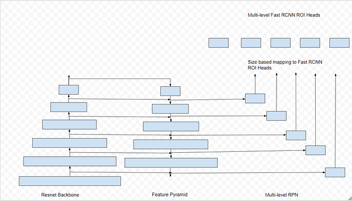
The following diagram depicts the basic essences of Faster-RCNN with FPN. The Feature Pyramid network up samples and mixes features from a number of layers in the backbone. Each of these levels of the pyramid can capture objects of various sizes — this is what supposedly provides the increased accuracy in FPN. The features output from different levels feed into different RPN networks. These RPNs generate region proposals of various sizes. The RPNs share parameter value. Based on the size of the proposal, they are fed into one of the the multi-level Fast-RCNN heads. All the Fast-RCNN heads also share parameter values. The sharing of parameter values in both the RPN and Fast-RCNN results in a lighter network with less parameters than otherwise.

When the number of levels in FPN is 0, then the network becomes similar to Faster-RCNN, with features taken directly out of the backbone network output.
For training the network end-to-end, both multilevel RPN and multilevel Fast-RCNN losses are added. Both of these losses usually have a class component and a regression component. The class component is usually cross-entropy loss and the regression component is usually Huber or Smooth L1 loss, etc losses (see for example [4] ). For more detailed description of Faster-RCNN see [2, 13]
Seq2Seq, Encoder-decoder, and Transformer Architecture overview:
Seq2seq converts one sequence into another for language translation, summarization , etc. Seq2seq often is based on RNN based encoder and decoder. The encoder-decoder architecture has been extensively used in Natural Language Processing (NLP) . At a high level level, encoder generates a representation context tensor from the input, the decoder then uses this context tensor ( and preceding outputs in the sequence) to generate a translated version of the input. In that sense the encoder-decoder architecture is very similar to auto-encoders used in computer vision.
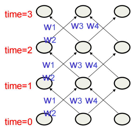
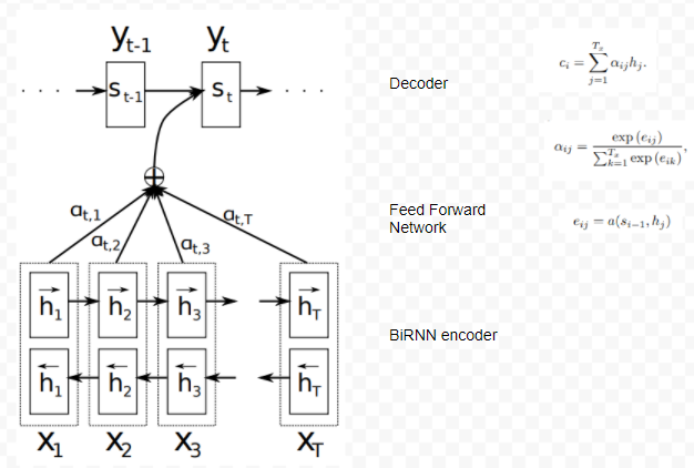
The problem with the simple encoder-decoder network is that all the information of the input is compressed into a smaller tensor. This makes it hard to handle long sentences, as all the possible nuances of every sentence possible needs to be captured in this single tensor. Another thing to note is that all intermediate tensors are thrown away, hence not used by the decoder. The attention mechanism was first proposed in [6] to improve RNN based encoder-decoder performance and used the intermediate results. The decoder uses attention to “focus” around a word in the input sequence, and thus have a much larger space to work with in comparison to the single context tensor. They showed effectiveness of attention mechanism on an encoder based on bidirectional RNN (BiRNN) with 1000 hidden units. For a refresher on RNN for example see [7]. RNNs sort of looks like Finite State Machines, but are much more capable as they have distributed weights. Another way to view RNN’s is that they are just a layered feed forward net that keeps reusing the same weights as shown the following diagram.

A BiRNN consists of forward and backward RNN’s. The forward RNN, f, reads the input sequence in order (from x1 to xt ) and calculates a sequence of forward hidden states ( fh1, · · · , fht). The backward RNN, b, reads the sequence in the reverse order (from xT to x1), to generate hidden states ( bh1, · · · , bht). They obtained an annotation for each word in the input sequence by combining the forward and backward hidden states [fh|bh] and applying a function called alignment. The alignment function models how well the inputs around position j and the output at position i match. Thus the annotation contains summaries of all the words in the sequence — both preceding and following the word. They used a feed forward network for alignment. The following figure shows the attention mechanism used in RNN. Some good media on broader aspect of attention are [9,10]. In a way, attention defines a network that is created on the fly that is based on the data it is seeing.

The next leap in NLP came with the Transformer architecture [5], shown in the following diagram. Transformers only uses attention without any sequence based networks such as RNN. However there is some similarity between previous RNN based diagram and Transformers. Here instead of RNNs, encoder and decoders are large blocks of tensor based attention operations, stacked in a number of units. Also the weights can be different in each unit unlike RNNs. The encoder through the Feed Forward Network feeds attention into the decoder. Both the encoder and decoder also uses self-attention, which essentially means all the input to the attention network is coming from within the encoder or decoder.

The authors incorporated attention in 3 different places — in encoder and decoder with all of Q,K,and V coming from the same source; between encoder and decoder with K and V coming from encoder and Q coming from decoder. Q, K and V vectors are produced by multiplying the input embedding or output of previous layer by a matrices that are learned. The input embeddings themselves are produced from the input text sequence.
Q, K and V can be looked at as a database with key and value pairs that is queried for an output.
There is no builtin sequence or ordering mechanism as in RNN, as all of the input is fed in one go. All parts of the input can thus be influenced by other part of input. In languages, sequence or order is a very important aspect ( e.g training a translating system vs a translating training system has completely different meaning). The authors incorporates ordering in Transformers by adding something called positional encoding at the bottom of encoder and decoder. They choose one sine and one cosine function of different frequencies for encoding position.
Good reviews of Transformers are towards the end of [11], and in [12].
Detection Transformer (DETR):
The following diagram shows the high level block diagram of DETR network.

The similarity between Faster-RCNN and DETR ends pretty much at the backbone used for feature extraction. Rest of DETR is based on the Transformer architecture [5]. The Transformer architecture has pretty much replaced LSTM/RNN in sequence prediction tasks and is used heavily in Natural Language Processing (NLP).
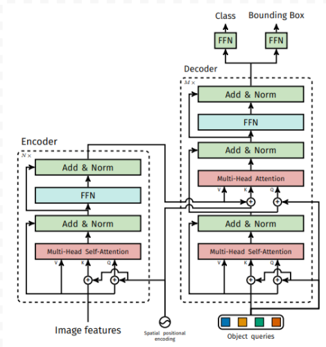
The following figure shows the DETR Transformer architecture with Encoders and Decoders.

The data flows through DERT’s network as follows. The bracketed notation indicates shape of tensors. The various tensors are named accordingly : pos for position embedding , feature for features from the backbone, . The input to the backbone is a batch of RGB images.
Backbone Input/Input image — [4, 3, 1216, 704] # batch,channel,w,h
Backbone output — feature [4, 2048, 38, 22], pos [4, 256, 38, 22]
Transformer input — projected_feature [4, 256, 38,22 ], mask [4, 38, 22], query [100, 256] , pos [4, 256, 38, 22]
Encoder input — src [836, 4, 256], mask [4, 836], pos [836, 4, 256]. src is derived from projected_feature , and the rectangular feature is flattened into a line ( e.g. 38*22 = 836) .
Encoder output — memory [836, 4, 256]
Decoder input — tgt [100, 4, 256], memory [836, 4, 256] , mask [4, 836], pos [836, 4, 256], query_embed [100, 4, 256]
Decoder output — hs [6, 100, 4, 256]
The q,k, and v to the encoder self-attention layer are simply src+pos, src+pos , and src respectively. In the above, src is derived from projected_feature .
The q,k and v to the decoder self-attention layer are tgt+pos, tgt+pos, and tgt respectively. Tgt tensor is set to all 0s during every iteration.
The q,k and v to the decoder multihead cross-attention are tgt-norm1+query_pos, memory+pos, and memory respectively. query_pos is entirely derived from query_embed. query_embed is a learned positional embedding, it gets updated every iteration during training. tgt-norm1 is the output from the norm layer of self-attention.
The output from the decoder is taken through a linear and a MLP layer respectively to generate the class and bounding box output.
The loss calculation in DETR is somewhat unique with the use of Hungarian Matcher and IoU. A Hungarian matcher is used to find the most probable bounding boxes from the model with respect to the target. Hungarian algorithm is well known combinatorial optimization technique. The loss function computes losses over the matched bounding boxes, composing of class loss and box loss as in Faster-RCNN. The class loss is a cross-entropy loss as in Faster-RCNN. The bounding box loss is slightly different in that it is a linear combination of L1 loss and generalized IoU loss. All the 3 losses — cross entropy, bounding box L1 and bounding box GIoU are weighted and added to produce the final loss.
Epilogue:
It is apparent from the above that the architecture of DETR is significantly simpler than even vanilla Faster-RCNN. In Faster-RCNN, lot of complexity is around RPN. Another difference to note is that there is no NMS as in Faster-RCNN. A third difference is that no cropping as in the detection stage of Faster-RCNN. A fourth difference is in how the final loss is computed. In addition to the layer architecture, loss calculation is another dimension where networks can differ significantly.
In Faster-RCNN and its predecessors, influence of classical computer vision techniques were still visible. Windowing being the most prominent. Broadly speaking anchors are a form of windowing. Secondly, a number of selected windows are then more closely examined before NMS is applied for final output. DETR completely moves away from that approach. The pixel features become analogous to work tokens in a sentence. In language models, attention layer establishes any to any relationship between embedded word tokens. Similarly, in DETR any to any relationship between the pixel features are also established by the attention layers. Which then produces the class and bounding box as final output.
References:
- End-to-end Object Detection with Transformers, https://ai.facebook.com/research/publications/end-to-end-object-detection-with-transformers
- Faster R-CNN: Towards Real-Time Object Detection with Region Proposal Networks, https://arxiv.org/abs/1506.01497
- Feature Pyramid Networks for Object Detection, https://arxiv.org/abs/1612.03144
- tensorpack, https://github.com/tensorpack/tensorpack .
- Attention Is All You Need, https://arxiv.org/pdf/1706.03762.pdf
- NEURAL MACHINE TRANSLATION
BY JOINTLY LEARNING TO ALIGN AND TRANSLATE, https://arxiv.org/pdf/1409.0473.pdf - CSC2535 2013: Advanced Machine Learning Lecture 10, Recurrent neural networks, https://www.cs.toronto.edu/~hinton/csc2535/notes/lec10new.pdf
- LSTM is dead. Long Live Transformers, https://www.youtube.com/watch?v=S27pHKBEp30
- Deep Learning 7. Attention and Memory in Deep Learning, https://www.youtube.com/watch?v=Q57rzaHHO0k
- DeepMind x UCL | Deep Learning Lectures | 8/12 | Attention and Memory in Deep Learning, https://www.youtube.com/watch?v=AIiwuClvH6k
- CMU Neural Nets for NLP 2020 — Lecture 7 : Attention — https://www.youtube.com/watch?v=jDaJYOmF2iQ&list=PL8PYTP1V4I8CJ7nMxMC8aXv8WqKYwj-aJ&index=6
- The Illustrated Transformer, http://jalammar.github.io/illustrated-transformer/
- A deeper look at how Faster-RCNN works, https://medium.com/@whatdhack/a-deeper-look-at-how-faster-rcnn-works-84081284e1cd
