A deeper look at how Faster-RCNN works
Faster-RCNN is one of the most well known object detection neural networks [1,2]. It is also the basis for many derived networks for segmentation, 3D object detection, fusion of LIDAR point cloud with image ,etc. An intuitive deep understanding of how Faster-RCNN works can be very useful.
The 3 networks of Faster-RCNN
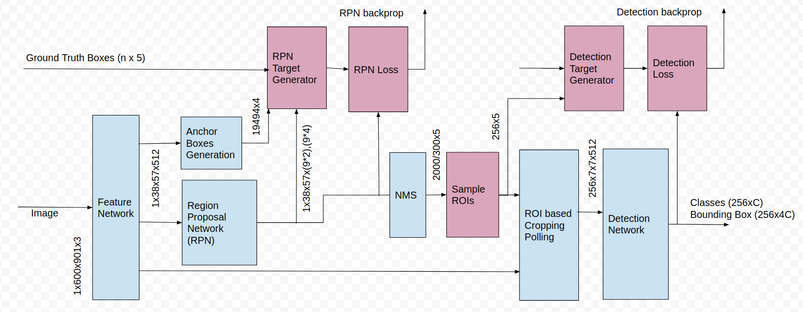
At the conceptual level, Faster-RCNN is composed of 3 neural networks — Feature Network, Region Proposal Network (RPN), Detection Network [3,4,5,6].
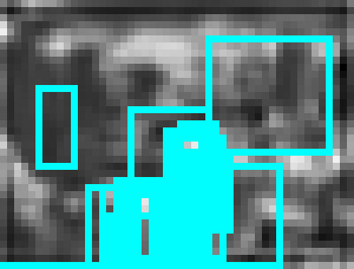
The Feature Network is usually a well known pre-trained image classification network such as VGG minus a few last/top layers. The function of this network is to generate good features from the images. The output of this network maintains the the shape and structure of the original image ( i.e. still rectangular, pixels in the original image roughly gets mapped to corresponding feature “pixels”, etc.) Fig 1 and Fig 2.


The RPN is usually a simple network with a 3 convolutional layers. There is one common layer which feeds into a two layers — one for classification and the other for bounding box regression. The purpose of RPN is to generate a number of bounding boxes called Region of Interests ( ROIs) that has high probability of containing any object. The output from this network is a number of bounding boxes identified by the pixel co-ordinates of two diagonal corners, and a value (1, 0, or -1, indicating whether an object is in the bounding box or not or the box can be ignored respectively ).
The Detection Network ( sometimes also called the RCNN network ) takes input from both the Feature Network and RPN , and generates the final class and bounding box. It is normally composed of 4 Fully Connected or Dense layers. There are 2 stacked common layers shared by a classification layer and a bounding box regression layer. To help it classify only the inside of the bounding boxes, the features are cropped according to the bounding boxes.
Both the RPN and Detection Network needs to be trained. This is where most of the complexities of Faster-RCNN lies.
Training the RPN
For training the RPN, first a number of bounding boxes are generated by a mechanism called anchor boxes. Every ‘pixel’ of the feature image is considered an anchor. Each anchor corresponds to a larger set of squares of pixel in the original image ( some reshaping is usually done on the original image before feature extraction). As can be seen in Fig 3 , anchors are positioned uniformly across both dimensions of the (reshaped) image. The input that is required from the feature generation layer to generate anchor boxes is the shape of the tensor, not the full feature tensor itself.
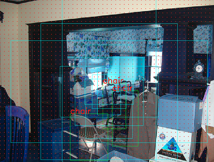
A number of rectangular boxes of different shapes and sizes are generated centered on each anchor. Usually 9 boxes are generated per anchor (3 sizes x 3 shapes) as shown in Fig 4. Hence, there are 10s of thousands of anchor boxes per image. For example in Fig 1, 38x57x9 = 19494 anchor boxes are generated.
In the fist step of reduction an operation called Non-Maximum Suppression ( NMS) is used. NMS removes boxes that overlaps with other boxes that has higher scores ( scores are unnormalized probabilities , e.g. before softmax is applied to normalize). About 2000 boxes are extracted during training phase ( the number is lower, about 300 for testing phase). In the testing phase these boxes along with their scores go straight to the Detection Network. In the training phase the 2000 boxes are further reduced through sampling to about 256 before entering the Detection Network.
To generate labels for RPN classification ( e.g. foreground , background , and ignore ), IOU of all the bounding boxes against all the ground truth boxes are taken. Then the IOUs are used to label the 256 ROIs as foreground and background, and ignored. These labels are then used to calculate the cross-entropy loss, after first removing the ignored (-1) class boxes.
In addition to classification, the RPN also tries to tighten the center and the size of the anchor boxes around the target. This is called the bounding box regression. For this to happen, targets needs to be generated, and losses needs to be calculated for back propagation. The distance vector from the center of the ground truth box to the anchor box is taken and normalized to the size of the anchor box. That is the target delta vector for the center. The size target is the log of the ratio of size of each dimension of the ground truth over anchor box. The loss is calculated by using an expression called Smooth L1 Loss .
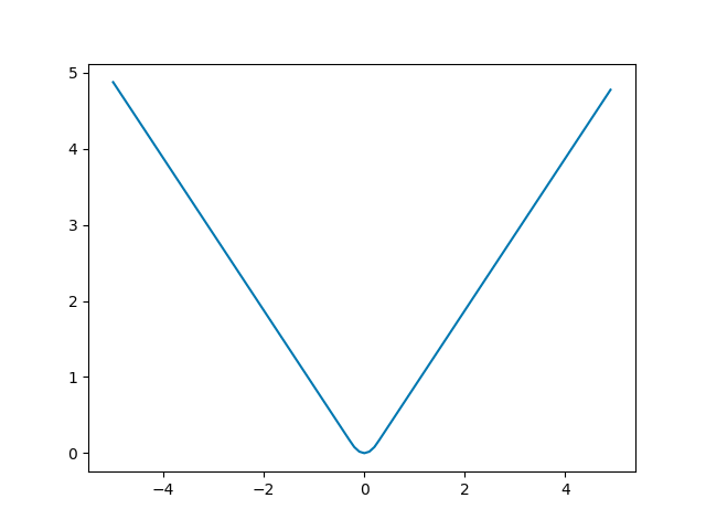
The regular L1 loss ( e.g. the norm or absolute value) is not differentiable at 0. Smooth L1 Loss overcomes this by using L2 loss near 0. The extent of L2 loss is tuned by a parameter called sigma. Mathematically the formula looks like the following pseudo-code. Fig 5 shows a plot of Smooth L1 loss vs the norm (d).
if abs(d) < 1/sigma**2
loss = (d*sigma)**2 /2
else
loss = abs(d) — 1/(2*sigma**2)
The losses are back propagated the usual way to train RPN. The RPN can be trained by itself, or jointly with the Detection Network.
Training the Detection Network
The Detection Network can be considered the removed layers (top ) of the classification network that is used for features generation. Hence the starting weights can be pre-loaded from that network before training.
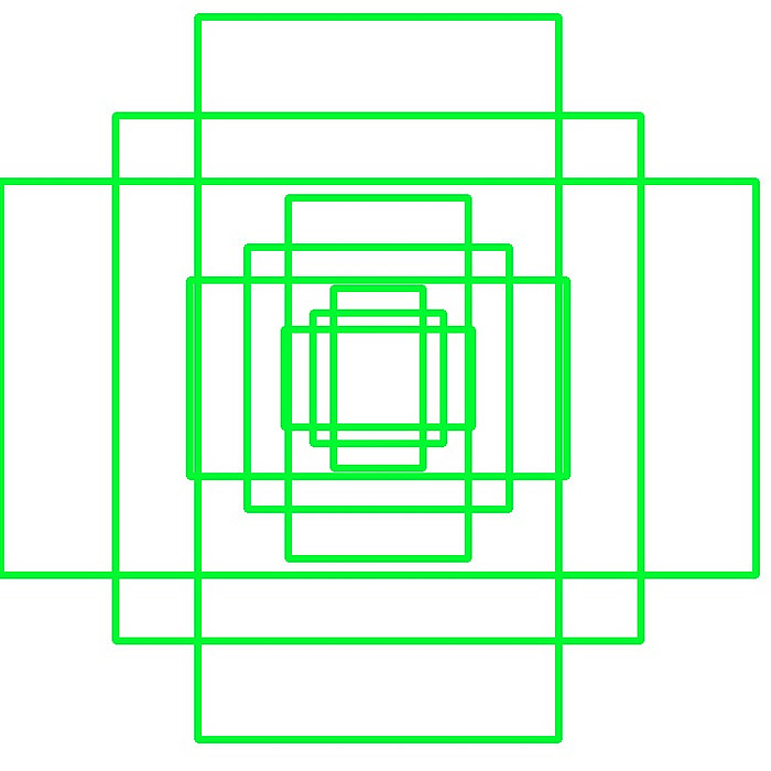
Training the Detection Network is similar to that of RPN. First, IOUs of all the 2000 or so ROIs generated by the NMS following RPN against each ground truth bounding box is calculated. Then the ROIs are labeled as foreground or background depending on the corresponding threshold values. Then a fixed number ( e.g. 256 ) ROIs are selected from the foreground and background ones. If there are not enough foreground and/or background ROIs to fill the fixed number, then some ROIs are duplicated at random.
The features are cropped ( and scaled ) to 14x14 (eventually max-pooled to 7x7 before entering the Detection Network ) according to the size of the ROIs (for this, ROI width and heights are scaled to the feature size). Fig 4 shows examples of ROIs overlaid on the feature image. The set of cropped features for each image are passed through the Detection Network as a batch.The final dense layers output for each cropped feature, the score and bounding box for each class ( e.g. 256 x C, 256x4C in one-hot encoding form, where C is the number of classes) .
To generate label for Detection Network classification, IOUs of all the ROIs and the ground truth boxes are calculated . Depending on IOU thresholds ( e.g. foreground above 0.5 , and background between 0.5 and 0.1), labels are generated for a subset of ROIs. The difference with RPN is that here there are more classes. Classes are encoded in sparse form, instead of one-hot encoding. Following a similar approach to the RPN target generation, bounding box targets are also generated. However, these targets are in the compact form as mentioned previously, hence are expanded to the one-hot encoding for calculation of loss.
The loss calculation is again similar to that of the RPN network. For classification sparse cross-entropy is used and for bounding boxes , Smooth L1 Loss is used. The difference with RPN loss is that there are more classes (say 20 including background) to consider instead of just 2 (foreground and background)
Conclusion:
There are 3 independent neural networks in Faster-RCNN — Feature Network, Region Proposal Network , and Detection Network. The complexity lies in training 2 out of the 3 — how to generate targets and labels, how to calculate loss, whether to train jointly or individually, etc.
References:
- Fast R-CNN, https://arxiv.org/pdf/1504.08083.pdf
- Faster R-CNN: Towards Real-Time Object Detection with Region Proposal Networks, https://arxiv.org/pdf/1506.01497.pdf
- https://github.com/rbgirshick/py-fase ter-rcnn
- https://github.com/facebookresearch/Detectron
- An Implementation of Faster RCNN with Study for Region Sampling, https://arxiv.org/pdf/1702.02138.pdf
- tf-faster-rcnn, https://github.com/endernewton/tf-faster-rcnn
